

Backtesting Introduction
On this page, the backtesting approaches and results are presented. All backtesting results start from January 1st, 2018, if available; otherwise, the earliest possible date is used. The backtesting is conducted in a fully mechanical manner, based solely on the signals generated by the trading strategy. Therefore, there is no room for emotional trading decisions.
Results Summary
The backtesting results are summarized in this section.
Strategy Approach
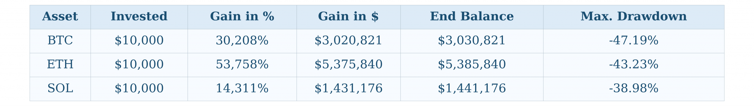
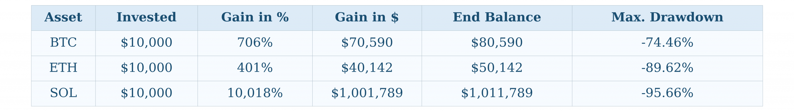
The table below shows the strategy approach performance for the three assets BTC, ETH and SOL. BTC and ETH were tested from 01/01/2018 until 01/11/2025. SOL was tested from 01/01/2021 until 01/11/2025.
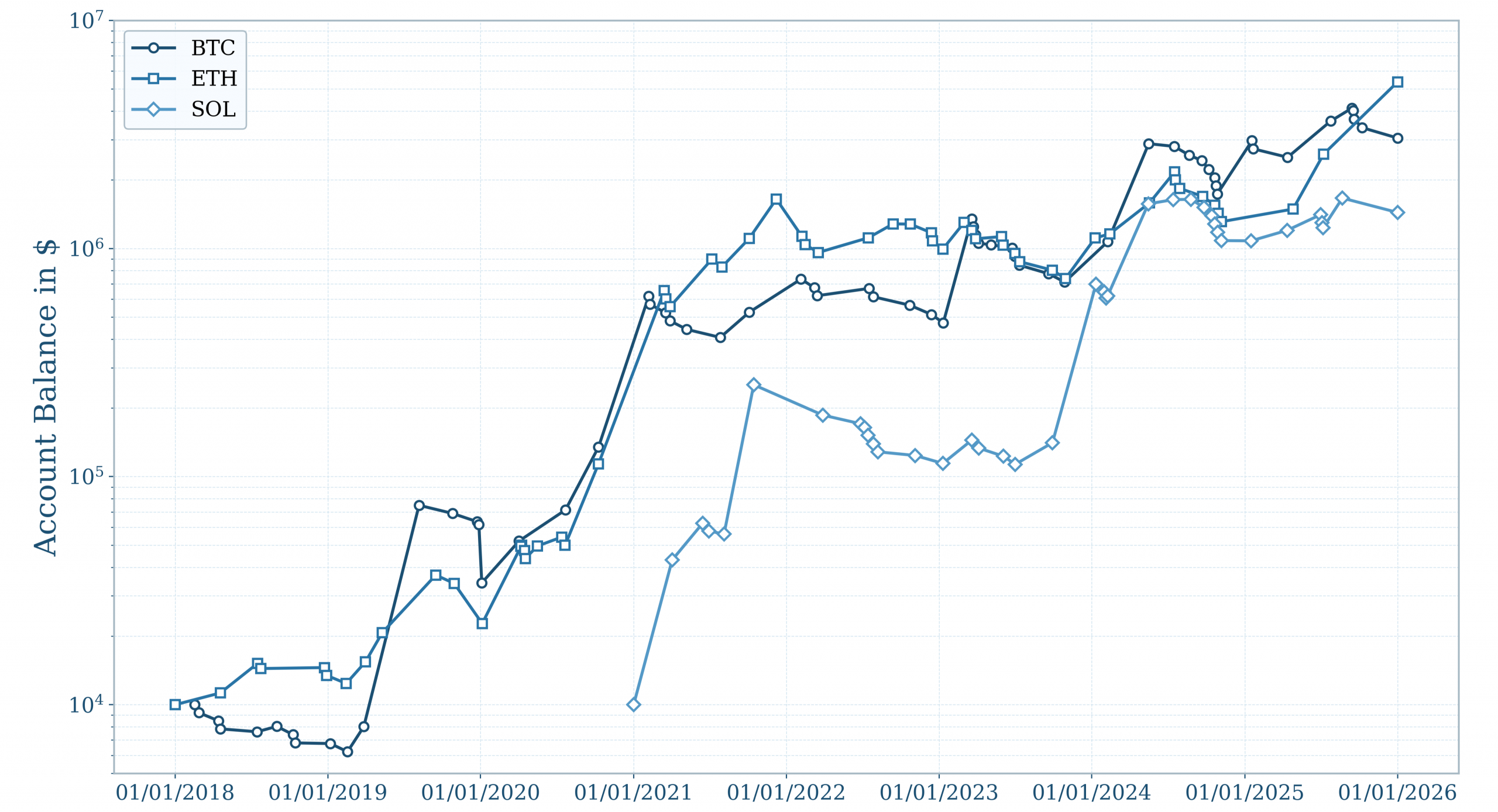
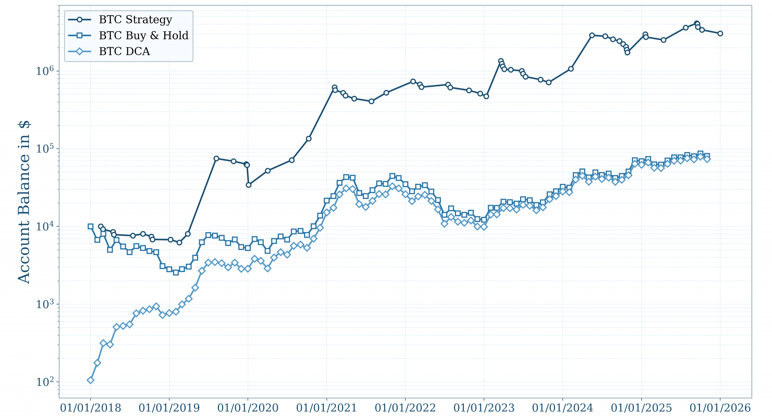
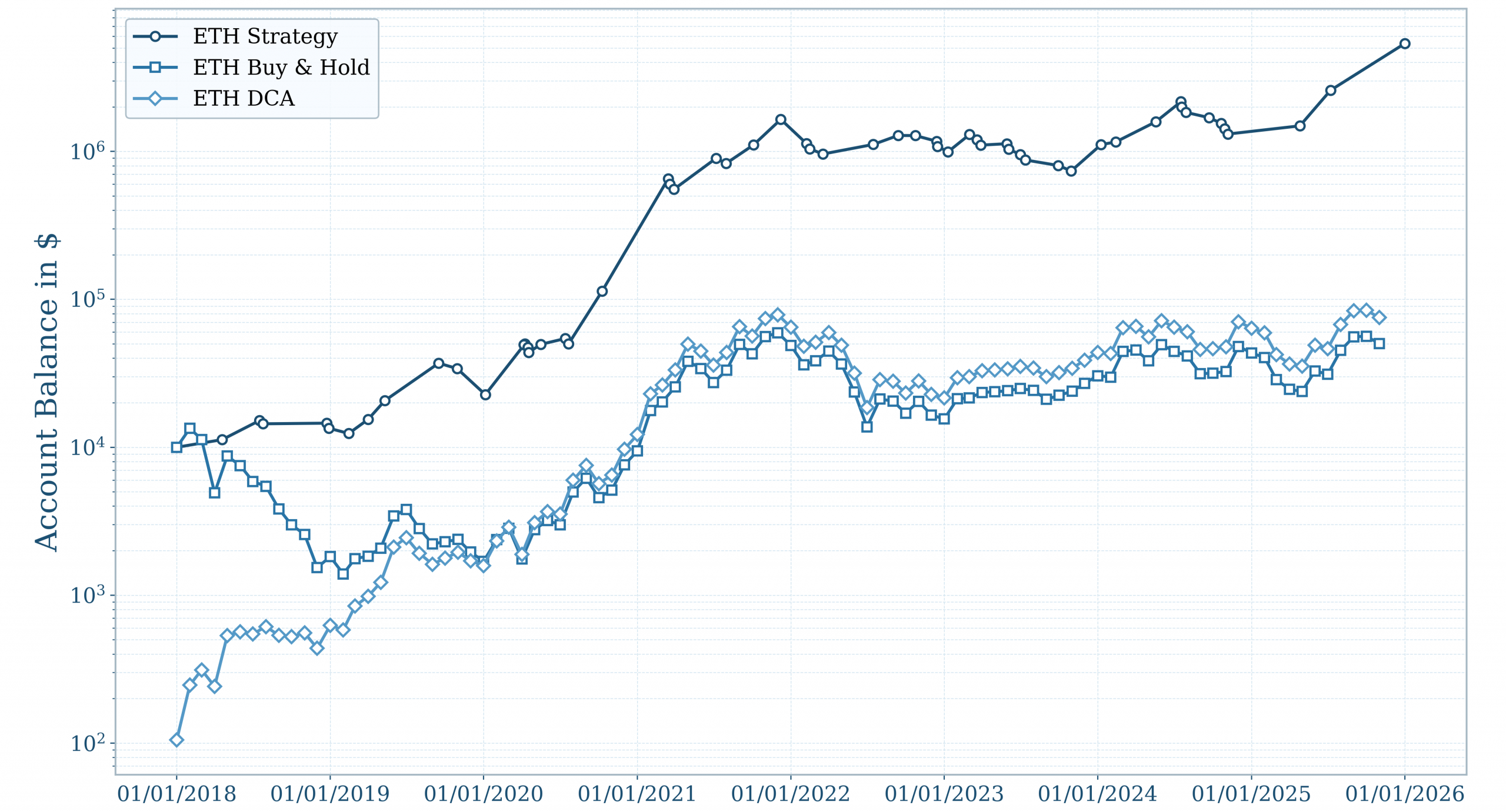
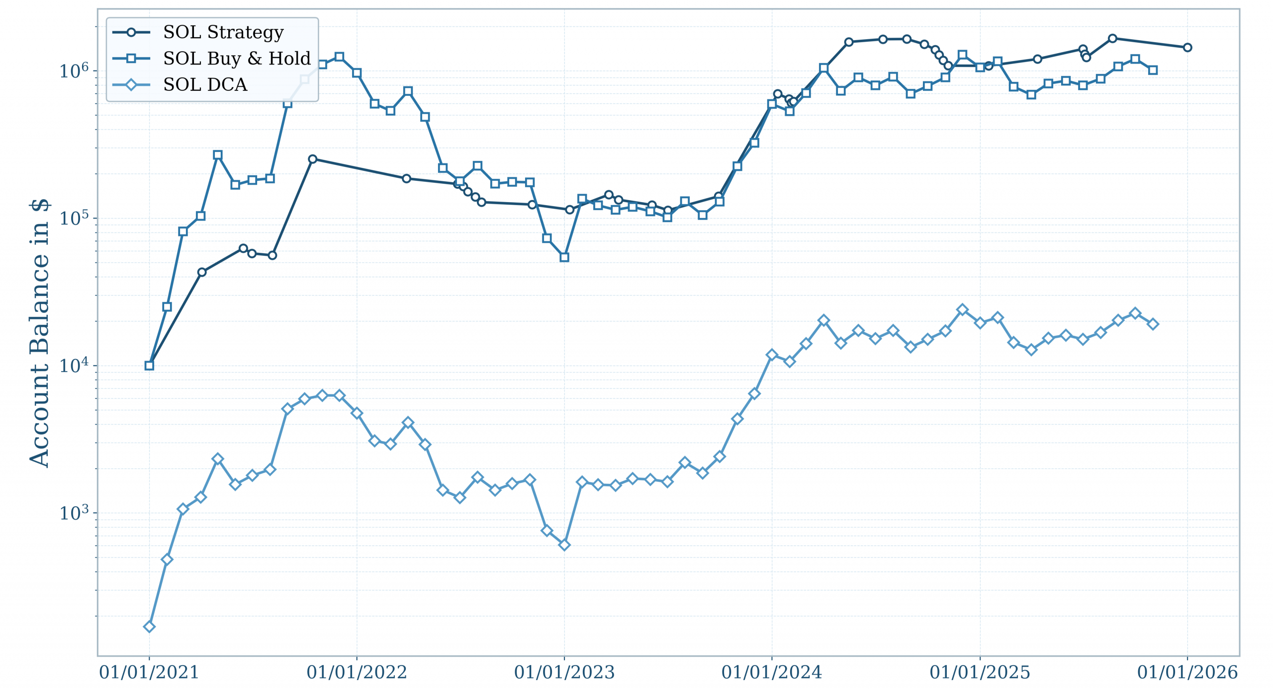
The diagram below shows the strategy performance over time for the three assets BTC, ETH and SOL.
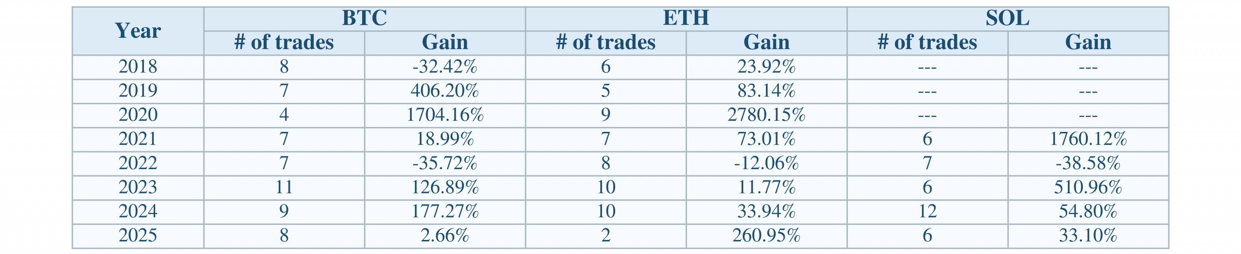
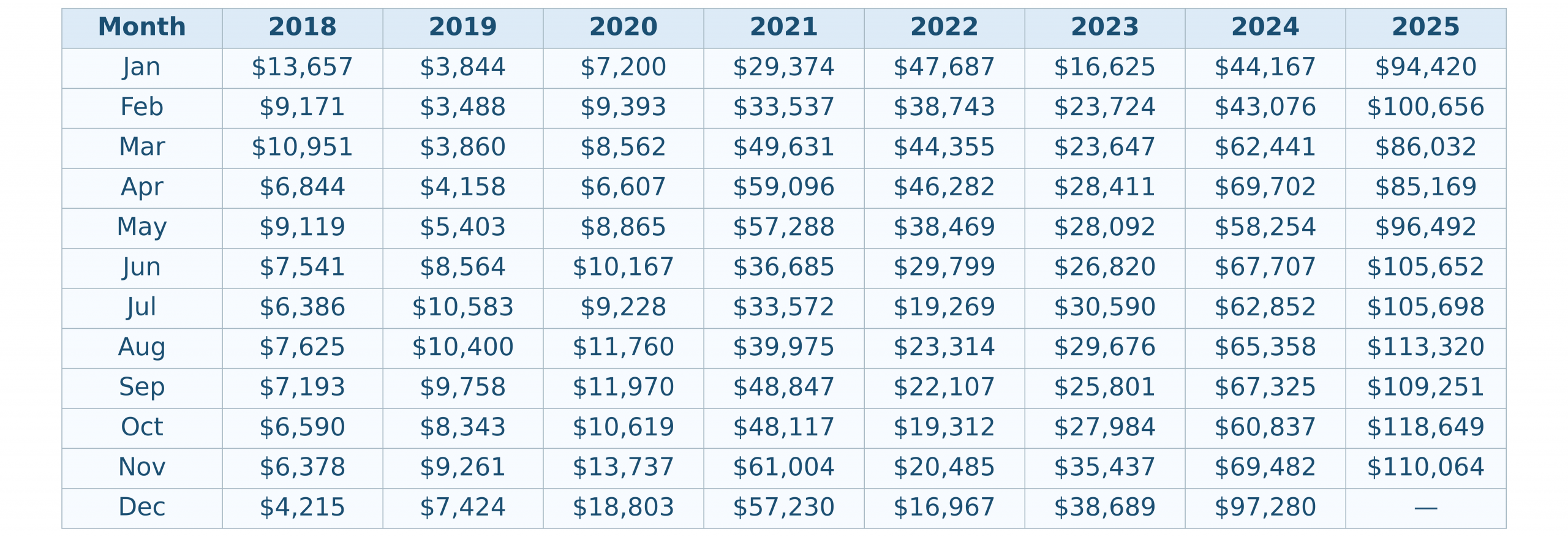
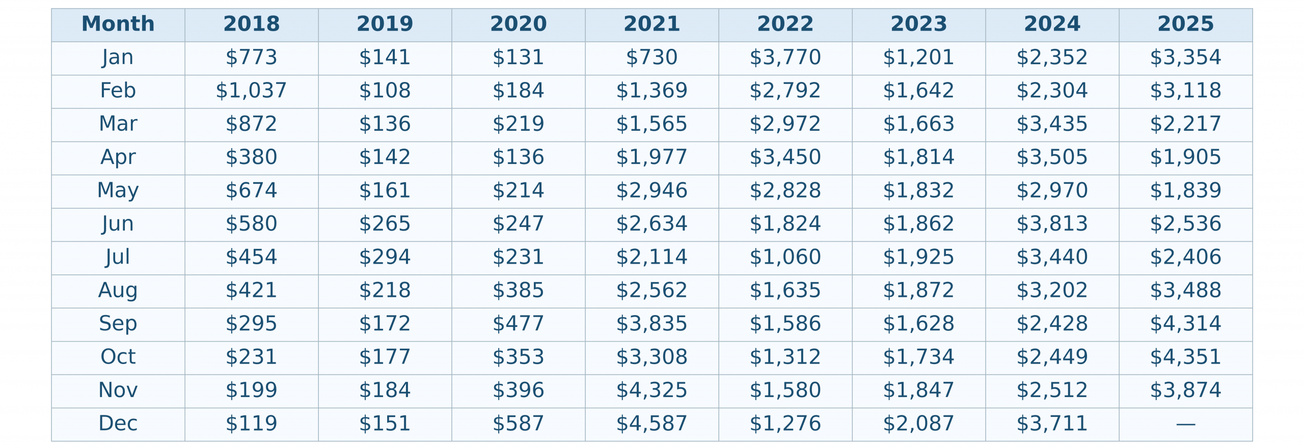
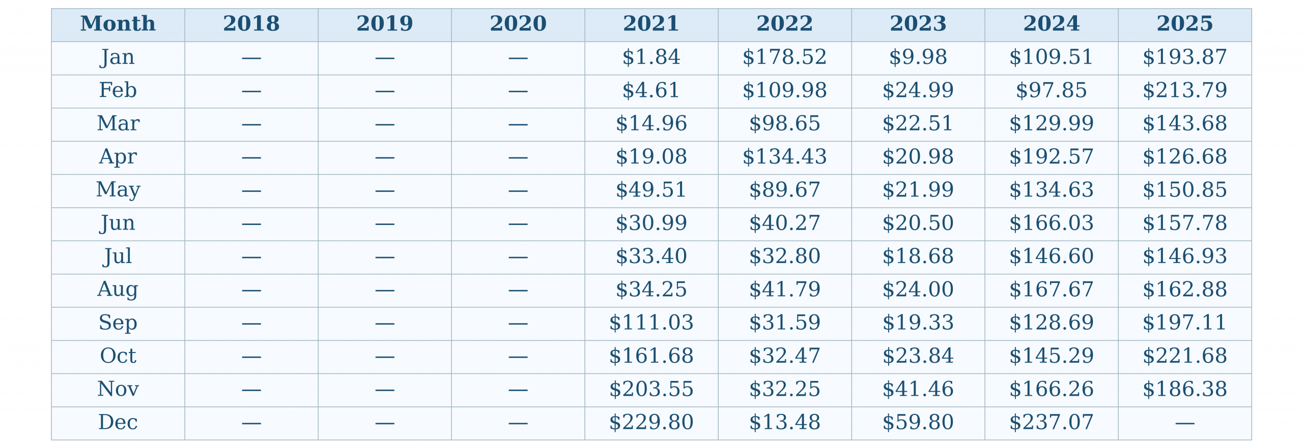
The following three tables show the performances over the years for the three assets BTC, ETH and SOL. Fees and taxes are included.
Additional strategy backtesting statistics are listed below.

Buy & Hold
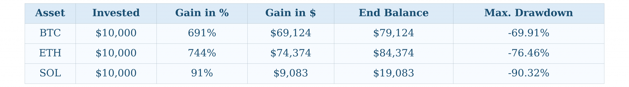
The table below shows the Buy & Hold approach performance for the three assets BTC, ETH and SOL.

DCA Approach
The table below shows the DCA approach performance for the three assets BTC, ETH and SOL.
Approach Comparison
Trading Fees
For realistic backtesting results, it is essential to consider trading fees. Since the strategy uses Spot-trading as well as Futures-trading, Maker-, Taker-, and Funding-fees apply. Additionally, worst case taxes need to be assumed.

For the backtesting, all fees are applied, also to Spot-trades. Hence, the total fees provide a potential upper bound. The resulting gains show a potential lower bound, respectively.
To provide an example, consider a Futures long-trade with a position size of $3,000 comprised out of a 3x leverage and a $1,000 balance. The trade runs for 60 days.
Maker- and Taker-fees:

Funding Fees:

Total Fees:

For this example, the total fees amount to $57.00. It is seen that the Funding-fees contribute significantly to the total fees. Hence, it is inevitable to consider all fees for the backtesting. Taxes are assumed once a year, if the PnL exceeded $1000 for that year. If the PnL is smaller than $1000 or if the PnL is negative for a certain year, no taxes are subtracted.
Backtested Approaches
In this section, the different approaches used for backtesting are presented.
Buy & Hold Backtest
The simplest approach is just lump sum at the beginning and hold. This approach is applied to the three assets BTC, ETH and SOL. It assumes an investment of $10,000 in the beginning, that is January 1st, 2018 for BTC and ETH and January 1st, 2021 for SOL. The results for this approach are shown in the table below.
A comment on the DCA approach: The results for SOL look very good in terms of total return. Nevertheless, it is highly unlikely to catch an asset at such an early stage. Therefore, these results should be interpreted with caution. Additionally, the maximum drawdown is unacceptably high.
DCA Backtest
One common investing approach is Dollar-Cost Averaging (DCA). At defined time intervals, a fixed amount of an asset is purchased — for example, investing $1,000 each month into an ETF. This strategy helps reduce the risk of buying at a local top, as might happen with a lump-sum investment. Nevertheless, the analysis in this and the following sections will show that, for single-asset investments, the potential reward can be significantly higher when timing the market compared to using DCA.
Assuming a time-span from January 1st, 2018 until November 1st, 2025, the BTC price for each first day of a new month were:
There were 95 investments.
For all backtests a total investment of $10,000 is assumed. Hence, in the DCA approach,  per month in case of BTC. For each month, one can calculate the amount of BTC purchased:

From this the accumulated amount of BTC is calculated. In the end, the total accumulated amount is multiplied with the current BTC price which results in the total account balance. Considering the BTC price as of November 1st, 2025 of $110,064, this results in an overall gain of 691%. In conclusion, having invested $105 per month since January 1st, 2018 resulted in a gain of 691%. The total investment of $10,000 would have become approx. $79,000. Since the DCA approach is traded without leverage, only Taker-fees would apply. Note that fees are not considered in the DCA approach which is in favor of the DCA approach.
The same concept is applied to the assets ETH and SOL. The table below shows the ETH prices from January 1st, 2018 until November 1st, 2025.
There were 95 investments.
The table below shows the SOL prices from January 1st, 2021 until November 1st, 2025.
There were 59 investments.
For the three assets shown above, the DCA approach leads to a gain as shown in the table below.

Strategy Backtest
The backtesting results derived from the applied trading strategy are presented in this section. As all trades were held for less than one year, the resulting profits are subject to taxation. The tax assumptions are based on the German taxation framework, applying an approximate upper tax rate of 45%, as outlined previously. In principle, taxes become relevant only when annual gains exceed a defined exemption threshold. However, for the sake of simplification — and to provide a conservative lower bound for net performance—taxes are applied as soon as any profits are realized.
In contrast to the DCA approach, funding fees are applicable and have been incorporated into the overall performance calculations. The total return and maximum drawdown are highly sensitive to the assumed loss threshold per trade. In the baseline configuration, a 7.5% loss limit per trade is employed, which can be regarded as relatively aggressive. Given that the three assets (BTC, ETH, and SOL) are each allocated 33% of the total account balance, a single trade corresponds to a potential maximum loss of approximately 2.5% relative to the total balance. Nevertheless, if three trades are executed simultaneously, the cumulative loss in the worst-case scenario could amount to 7.5% of the total account balance. To compute the account balance and gains/losses over time, the following calculations are made.
Leverage, Total Gain in %, Amount used for Trade and Position Size:

Net Gain:

Again, an example is used to demonstrade the calculations. Let’s assume an account balance of $10,000 of which 33% are used for the trade. A winning trade with a gain of 15 % is assumed. The %-to-Stop-Loss value is 3 %. The trade was opened for 50 days.
First, the leverage is calculated as follows:

The amount used for the trade is:

The total gain in % considering the previously calculated leverage is:

The position size amounts to:

The resulting new account balance is:
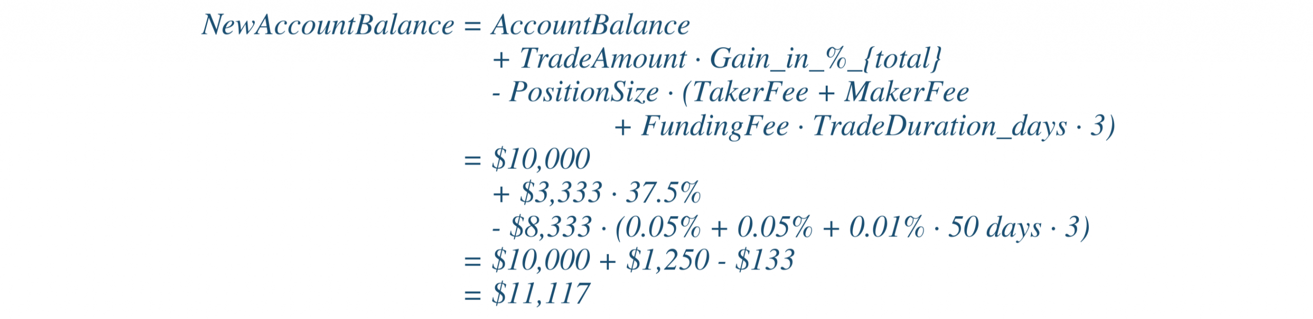
From the calculations shown above, the trade resulted in a gross gain of $1,250. $133 in fees had to be paid which leads to a net gain of $1,117. Since compounding is used for the backtests, the new account balance of $11,117 would be considered for the next trade.
The complete backtesting results and the formulas applied in the tables can be found at BTC Complete Backtesting Results, ETH Complete Backtesting Results and SOL Complete Backtesting Results. Based on the backtesting results, the strategy approach leads to a gain as shown in the table below. The initial balance is set to $10,000. Other than in the example, the full account is used for the trades, to be able to compare them to the DCA-approach.
