This section outlines a cross-sectional momentum strategy designed to allocate capital systematically across a universe of crypto assets. Rather than focusing on the direction of a single asset, the system evaluates the relative performance of multiple cryptocurrencies and constructs positions based on their comparative strength and weakness.

The strategy is built on the premise that assets with stronger recent performance tend to continue outperforming in the short term, while relatively weaker assets often remain under pressure. By ranking assets according to their recent returns, the system simultaneously establishes positions in both the strongest and weakest performers, seeking to capture relative price dispersion within the crypto market.

In addition, the strategy distinguishes between bullish and bearish market environments. Depending on the prevailing regime, the portfolio adjusts its exposure to reflect the broader conditions of the crypto market, allowing the system to adapt its positioning while maintaining a consistent momentum-driven framework.

Because returns are generated through relative performance across assets, individual positions may offset one another within a given trading cycle. Portfolio performance is therefore driven by the persistence of momentum relationships across the asset universe rather than the direction of any single cryptocurrency.

All signals, portfolio construction, and position sizing are fully systematic and governed by a predefined rule set, ensuring that the strategy operates mechanically and without discretionary intervention.

In the following, the strategy is described using a simplified example with a set of hypothetical assets. The goal is to illustrate the core mechanics step by step, from signal generation to position selection and final performance.

In Step 1, each asset’s return is calculated over the lookback period $T_{\mathrm{Lookback}}$ to measure recent performance.

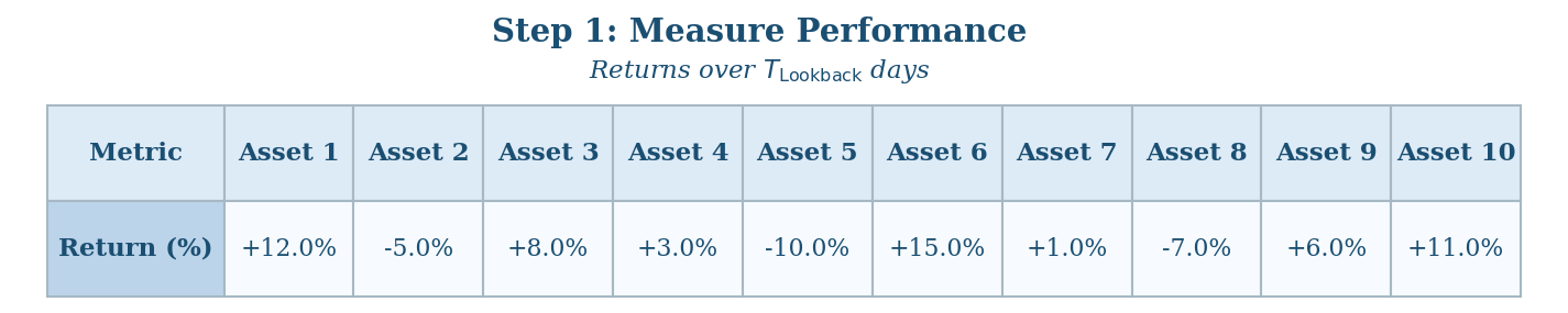
In this example, Asset 6 (+15%) and Asset 1 (+12%) show the strongest gains, while Asset 5 (−10%) and Asset 8 (−7%) are among the weakest.

n Step 2, all assets are ranked from highest to lowest return based on the results from Step 1. This ranking highlights relative strength and weakness.

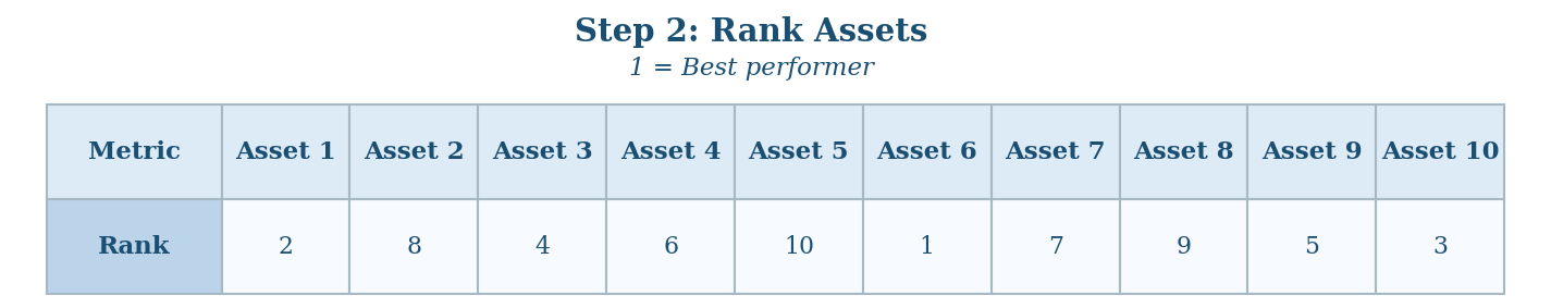
Here, Asset 6 is ranked 1st, followed by Asset 1, while Asset 5 is ranked last.

In Step 3, positions are assigned based on the ranking. The strongest assets are selected as long positions, while the weakest assets are selected as short positions.

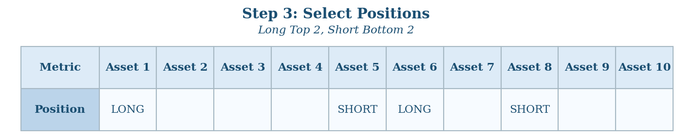
In this example, Asset 6 and Asset 1 are chosen as longs, while Asset 5 and Asset 8 are selected as shorts.

In Step 4, the selected positions are held for the period $T_{\mathrm{Holding}}$​, and their performance is evaluated. Long positions benefit from rising prices, while short positions benefit from falling prices.

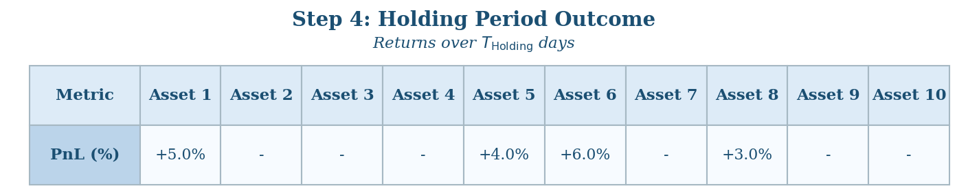
In this example:

• Asset 1 (long, +5%) → +5%
• Asset 6 (long, +6%) → +6%
• Asset 5 (short, +4%) → -4%
• Asset 8 (short, +3%) → -3%

Assuming an equal allocation for each position, the overall result is the average across all positions: (5% + 6% − 4% − 3%) / 4 = 1%. Although the short positions contributed negatively, the stronger performance of the long positions outweighed these losses, leading to a net gain at the portfolio level.

In addition to the steps shown above, the strategy adapts its exposure depending on the prevailing market environment. In a bullish regime, the number of long positions can be increased relative to short positions, while in a bearish regime, the allocation can shift towards more short positions. Such regime classification can be based on a long-term trend indicator, for example whether the price of a benchmark asset (e.g., BTC) is above or below its 200-day EMA. This allows the strategy to remain aligned with broader market conditions while maintaining its cross-sectional momentum structure.

This simplified example illustrates how the strategy translates relative performance into a systematic portfolio allocation. By ranking assets based on their recent returns over $T_{\mathrm{Lookback}}$​, positions are established in both the strongest and weakest performers, allowing the portfolio to capture differences in performance across the asset universe.

The resulting portfolio return, as shown in Step 4, is driven by the combined contribution of long and short positions rather than the absolute direction of individual assets. This reflects the core principle of the strategy: performance is generated through relative strength and weakness within the market, consistent with a cross-sectional momentum approach.